A lossy compression algorithm that learns features on-the-fly

Spring 2023 — Python & NumPy project

Example model features visualized on a dataset of celebrity faces.

Motivation

In this project, I designed an algorithm that mitigates some of the major shortcomings of modern deep learning methods. Two of these shortcomings are the following:

Deep learning algorithms are not great at learning from new data. Given a topic that was not in the training set, a deep learning algorithm would need to either a) keep the topic in its context, and use its existing weights to interpret the data, or b) fine-tune the model on the new topic. In the first case, the model doesn’t strictly learn from the topic, it instead uses what it has already learned in order to process the new topic without internalizing any of the new data. In the second case, we would need to retrain the model weights, while making sure that a) the model doesn’t lose performance on its previous data, and b) the model doesn’t overfit to the new training data by using a development set. This can get expensive, especially when dealing with larger models. Ideally, a generative model would be able to expand itself given the presence of new data without having to adjust all of its weights. I.e., it would be able to learn new features on-the-fly.
Deep learning algorithms are not easily interpretable. There is ongoing research in interpreting model activations, yet these methods are intricate and not always successsful. The internal representation of modern language models is a set of vectors in a high dimensional embedding space, where each value in a vector is not necessarily human-interpretable. There’s a great paper by Andrej Karpathy where he analyzes individual activations in an LSTM model in an attempt to understand the role of each activation in language modeling. Ideally, activations in a deep learning model would be easily interpretable, in that we would be able to identify exactly which parts of the model triggered the activation.

I designed this compression algorithm with those two points in mind.

Overview of Algorithm

The high level structure of the algorithm is as follows: first, the algorithm looks at an input datapoint and processes it with its existing features (think of this as the "forward pass" of the algorithm). Each feature can be thought of as a single "neuron", where the feature is only activated when enough of its input features are activated. Then, the algorithm examines which feature activations were used to activate other features in the model, and the algorithm collects all activations that didn't trigger some downstream activation for the input. Then, the algorithm creates a new feature that takes as input a subset of features from those features (the features that didn't trigger an activation). In other words, the model trains by interatively building features on-the-fly when it encounters input that isn’t cleanly captured by existing features.

To prevent overfitting/rote memorization, the model flips a biased coin to decide whether it should create a new feature from a subset of the candidate input features. This guarantees that patterns that occur more often are more likely to be captured as features in the model, and patterns that are rare are less likely to be captured by the model. This is especially useful when building the initial features, and after the model has built a base set of features, we can modify the coin’s bias in order to allow for faster learning. Additionally, we could include a “forgetting” phase where features that haven’t been seen for a long time will be removed from the model. This is also especially useful for the base set of features in order to limit the total computation of the lower levels of the model. As with the learning phase, we could reduce the amount of forgetting in the later stages of model traning in order to make sure we don’t forget high level features that, while rare, are still useful every once in a while.

I’d like to highlight the aspects of human learning that this algorithm mimics:

The model has the ability to learn new concepts very quickly.
The model might need to be exposed to a new concept repeatedly in order to fully internalize it (due to the random nature of feature creation). This is similar to human learning, in that sometimes it takes a few iterations of learning about a new topic in order to internalize it.
As with humans, we tend to forget concepts that we don’t use over a long period of time. In the model, this is useful in freeing up computation so that the model can learn efficiently. The same could be said for humans.
As the human brain develops, its capacity for memorization improves. Similarly, we increase the likelihood that the model creates a feature from its inputs as the model grows.
The activations are sparse, as opposed to dense like existing deep learning methods. In other words, most features are not activated given an input data point. Similarly, given sensory input, the human brain does not activate all of its neurons, rather a select few.

Pseudocode

The pseudocode of the algorithm is as follows:

Initialize the model as an empty set of features.
Iteratively loop through the training data.
For each training sample, do the following:
1. The sample is composed of a set of activations.
2. For each feature in the model, use the sample activations and previously activated features to determine whether the next feature is activated.
3. If a feature is used to activate a downstream feature, mark the upstream feature as “used”.
4. Flip a biased coin. If heads, do the following:
  1. Randomly sample a set of “unused” features (features not marked as “used”).
  2. Create a new feature from that set of features - the new feature will be activated when at least X% of the input features are activated.

Python Implementation

The algorithm can be implemented in a very simple (yet inefficient) manner in Python using NumPy:

num_features = 0
input_dim = 100
feature_dim = 5
features = np.zeros((num_features, feature_dim))
activation_threshold = 0.8
feature_creation_likelihood = 0.1

for sample in training_data: 
    activations = np.zeros(num_features + input_dim)
    activations[:input_dim] = sample
    unused_features = np.zeros(num_features + input_dim)
    for i in range(num_features):
        activations[i + input_dim] = activations[features[i]].mean() >= activation_threshold
        if activations[i + input_dim] == 1:
            unused_features[i + input_dim] = 1
            unused_features[features[i]] = 0

    if random.random() <= feature_creation_likelihood:
        if unused_features.sum() >= feature_dim:
            new_feature = np.random.sample(np.where(unused_features)[0], feature_dim)
            features.append(new_feature)

The above implementation assumes that feature activation is binary, but the implementation can be easily modified to include weights for features and activation values that are real-valued. Similarly, the hyperparameters can be modified to allow for larger features, slower training (by reducing the feature_creation_likelihood hyperparameter), and the forgetting phase can be implemented. We can also create features from sampling a fraction of the unused features instead of a fixed number of them.

Additionally, the above implementation is not very efficient. It loops through each feature for each training sample, giving it a runtime complexity of O(num_features^2) for a single data point. While numpy is fast at indexing arrays for an array of indices (e.g. the activations[features[i]] step), the overall approach is inefficient.

A More Efficient Implementation

We can improve the efficiency of the algorithm by exploiting its sparse nature. For a given input most features remain unactivated, so we can modify the implementation to only iterate over features that we think might be activated. For each activated feature, we can loop through its downstream features, and update their activation values. If a feature’s activation increases above the threshold after we update its activation, we can repeat the process of incrementing the activation of its downstream features.

In other words, our implementation can instead focus on “routing” activations. We can assign each thread an activation, then loop through all of the downstream features for an activated feature, update the feature’s activation value, and repeat the process when downstream features cross the activation threshold. This implementation can use a GPU’s high parallelization, and avoid computing activations of features that are fully turned off.

Adding to the list of ways that this algorithm mimicks the human brain, activations are routed by neurons in the brain in parallel, and the brain does not waste energy on neurons that have not received any input activation.

Adapting the model for images

If we want to adapt the above model for images, we can apply the features in the same manner as a convolutional network - we treat each patch of each input image as a separate data point, and build the base set of features for patches of the image only. Then, to ensure we can build features that span multiple patches, we can apply the algorithm on increasingly larger patches that include the lower-level features extracted from smaller patches. This resembles convolutional neural network architectures. Implicit in this description is that each feature not only has an activation, but a location, and we constrain features to only take in lower level features within a fixed distance of each other.

Using the Model for Data Compression

How can we treat this model as a compression algorithm? We can interpret each feature as “summarizing” the features below it. If a feature is activated, we can essentially compress the upstream features by describing them with the downstream activated feature. This compresses the features because instead of having to store the activations for the input features (which will require feature_dim units of information), we only need to store one activation value indicating that the downstream feature is activated, and we can infer that the input features must have been mostly activated since the downstream feature was activated. This demonstrates the lossy nature of this algorithm - while we know that the input features must have been activated, we don’t know which ones exactly, so we lose some information in the process of compressing the inputs.

In other words, the unused_features array ends up being exactly the compressed version of the input data, because it contains only features that were not “summarized” by other features in the model. This also highlights how the algorithm works - each new feature is created only from the most compressed representation of the input data. While we are not guaranteed to have fewer activated features in the unused_features array than in the input (and thus not necessarily compressing the input), if the unused_features array has many features then that indicates that the algorithm hasn’t finished training, as the input has more potential for compression. Ideally, the unused_features array will contain few activations, indicating that we’ve summarized our inputs with a small number of features.

Evaluation

I tested this algorithm as a proof-of-concept on the MNIST dataset and the CelebA faces dataset. This raises the question - how do we evaluate this model? Since the model doesn’t optimize a loss function directly, we can’t directly compute the perplexity of the model on a test set. Instead, I opted to examine how well the algorithm compressed inputs by reconstructing the inputs given the extracted high level features.

For each high level feature, we can employ a few different methods for reconstructing the lower level features captured by the feature.

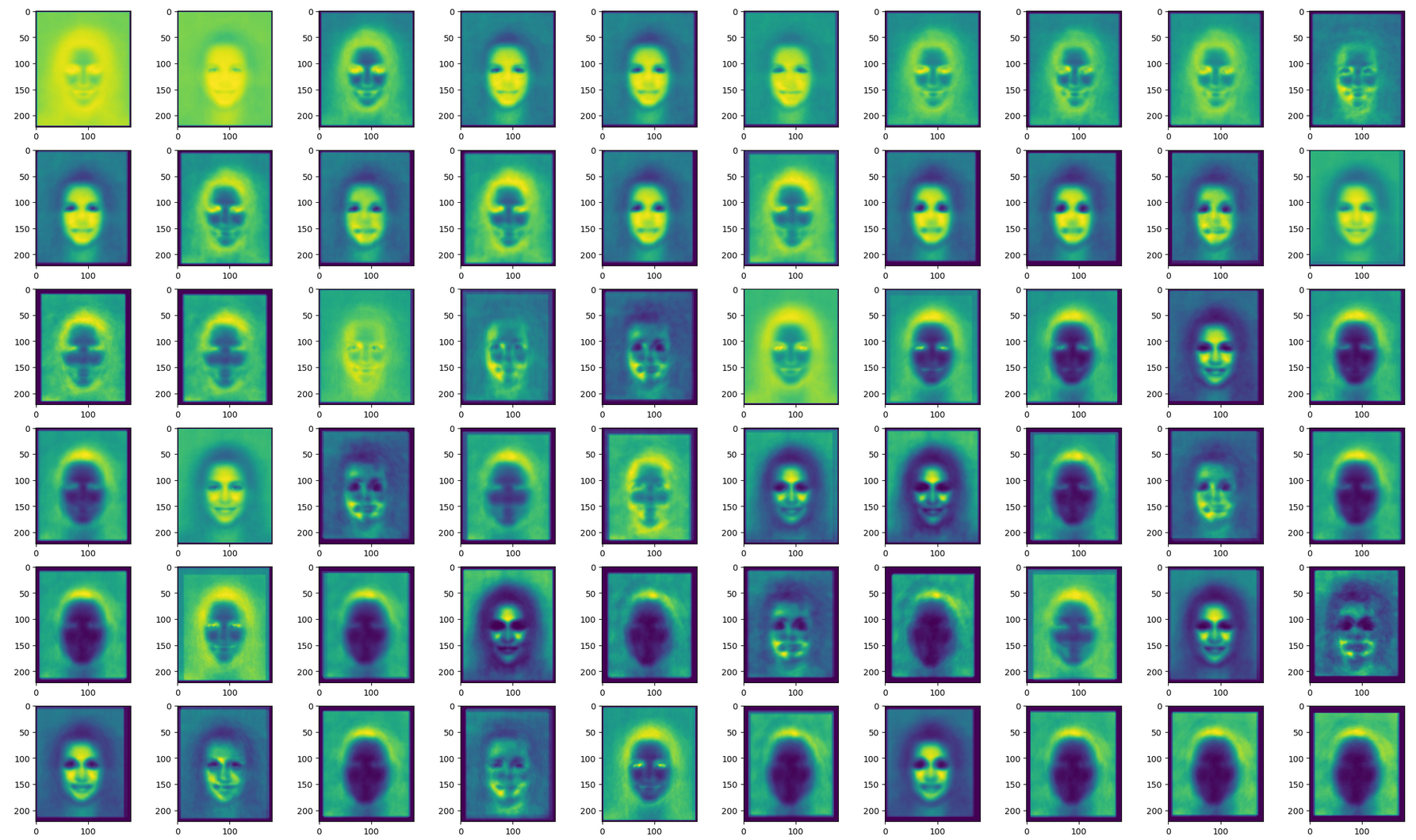
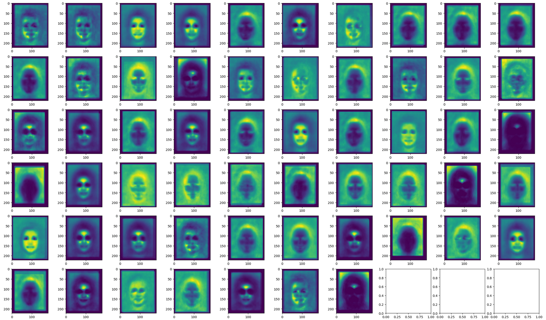
Anther way to interpret the algorithm's final features is to map out where the feature usually occurs in images. Given a dataset of faces that are all lined up in the same position, if we map out the usual locations of a feature we can get a sense of what part of the face the feature captures.

The following images show a sample set of features, and the locations that the feature tends to appear in. For each pixel, we color it more yellow if the feature tends to occur frequently at that pixel, and more blue if the feature tends to occur less frequently at that pixel. The first image contains a sample of features that are lower in the model, in that they aggregate less information. The second image is a sample of features constructed by combining intermediate features. Admittedly, the feature visualization is mildly haunting!

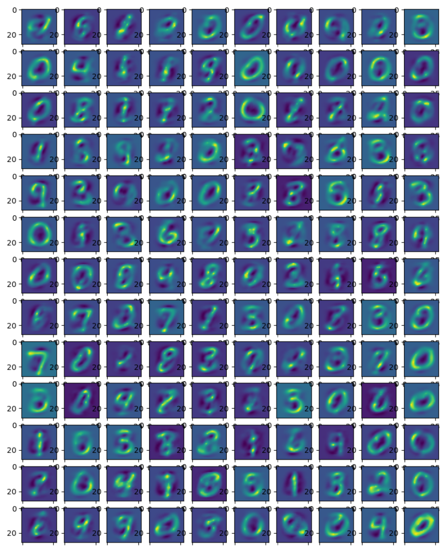
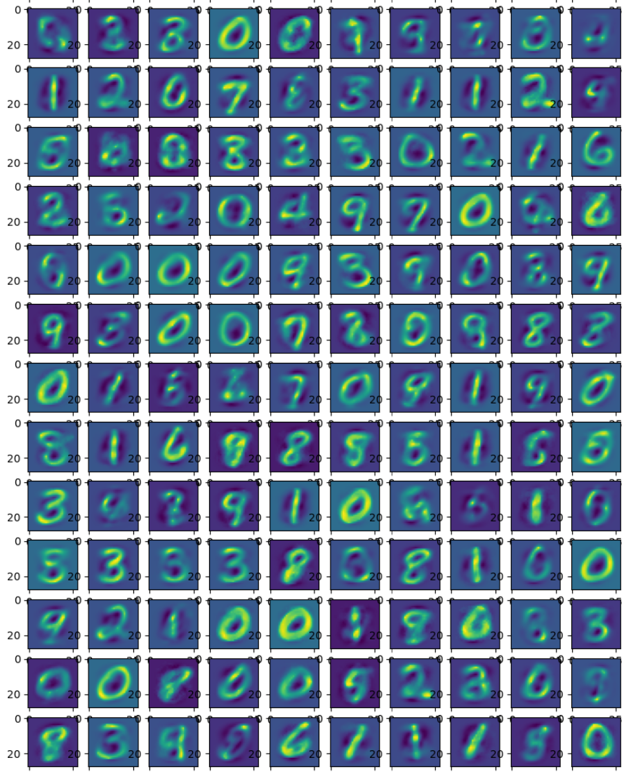
I repeated the above experiment on MNIST. The first image is of low level features, and the second image is of higher level features. Note that in this case, the higher level features look more like complete digits since they combine lower level features which tend to capture parts of digits.

One drawback of the algorithm is the prevalence of features that capture the same patterns, but do so using different parts of the same pattern. This can be mitigated by allowing for a variable number of feature inputs, so that if a large set of features occur frequently together, they can be captured by a single feature instead of multiple features of fixed size.

Future Testing

Closing Thoughts

Lastly, I’ll note that while this algorithm is interesting, it’s not obvious to me whether this algorithm is more cost-effective than existing deep learning models. My hunch is that the bitter lesson still applies, and regardless of the algorithm, getting to a specific level of performance with any generative model requires a certain amount of compute (an amount out of reach for the indie researcher).