Color hyperspheres for lossy image compression

June 2020 — Python & NumPy project

This project was inspired by Geoff Hinton’s work with capsule networks. Hinton’s goal is to develop computer vision algorithms that represent objects based on their 3D structure instead of high level color/texture pattern statistics as current models do. This project was a step in that direction: how can we extract basic building blocks for such algorithms from images? The goal of this project was to extract a kind of “generalized pixel” (pixels that vary in size and orientation) that could be used by downstream algorithms to identify objects based on their structure. While this project does not go beyond the first layer of feature extraction, it is nonetheless a interesting low-level way of processing images that doubles as a lossy compression algorithm.

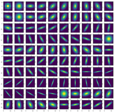
At the heart of the algorithm is the following problem: given a patch in the image, we want to identify whether a region of pixels of a specific shape conform to the same color. To keep the problem tractable, we restrict the regions to have the shape of 2D gaussians. The setup goes as follows: for each patch in the image, we aim to compute how closely the pixels in the patch match a given pattern. The following are the patterns we aim to detect in the image.

This problem resembles computing the convolution of an image and a filter, yet it differs in one crucial detail: the output of the computation on the patch should indicate how closely the color in the pixels matches a given pattern. Regular RGB space is not conducive to this task — if the mean pixel of a patch weighted by a gaussian is (128,128,128), then we don’t know whether the patch is entirely gray or whether the patch is comprised of many different colors that all sum to gray. In other words, convolutional filters don’t tell us anything about the variance of the pixels, and so are limited in extracting features for this task.

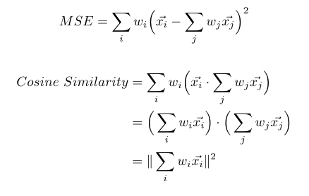
One naive approach we could is to compute the average pixel and then compute the mean difference from each pixel in the patch to the average, weighed by the filter weights. While this approach would work, it would require that we loop through all pixels in the patch for each patch, which would be quite inefficient. Another approach is to change the coordinate space so that we can utilize cosine similarity for such a task. If we compute the average vector for a patch and can take the dot product between the average vector and all other vectors in the patch, then we can distribute the dot product operation to simplify the expression. By doing so, the equation for how closely the patch matches the filter is merely the magnitude of the weighted mean of the patch. Equations for these two approaches are shown below, where the x’s are the patch pixels and the w’s are the filter weights.

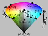
We’ve reduced the feature extraction computation to a simple convolution operation, which can be computed quickly using FFTs. All that remains is to map the pixels from RGB to a space conducive for dot product similarity scores. To do so, we first take the HSV representation of the pixels and map the 3D cone to a 3D sphere, which maps easily to one-half of the surface of a 4D hypersphere (a hyper-hemisphere). This coordinate space loosely resembles the color space defined in this paper on spherical color representations in the brain. The mapping is shown below, annotated atop the HSV color space.

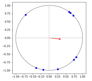
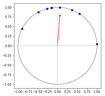
Mapping points to the surface of a hyper-hemisphere has a convenient property that all similarity scores are between -1 and 1. Just as with capsule networks, the direction of the extracted feature characterizes the feature, whereas the magnitude indicates how well the feature matched the observed data. The diagram below shows how the magnitude of average points on a circle increases when the points are closer together on the circle.

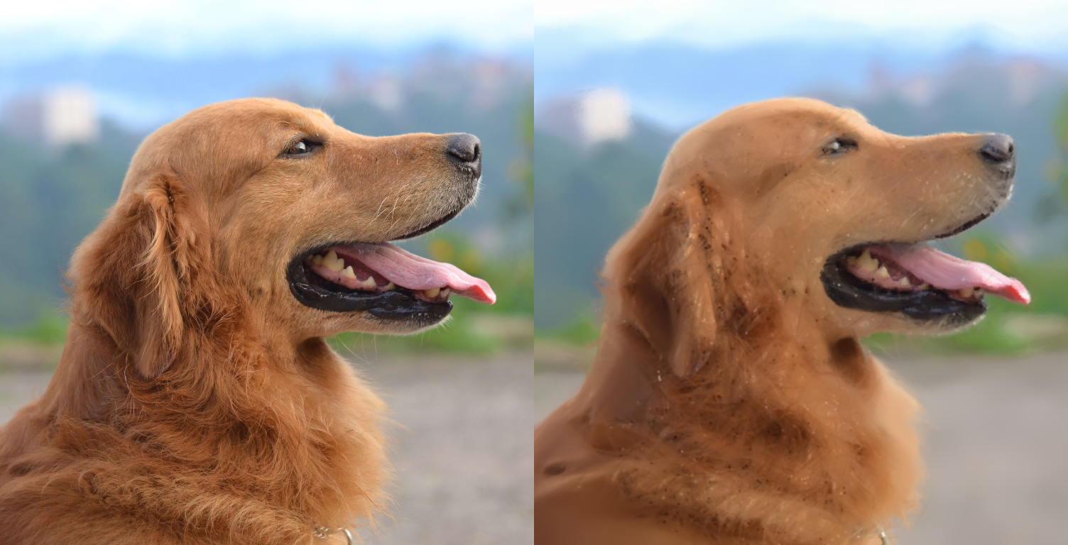
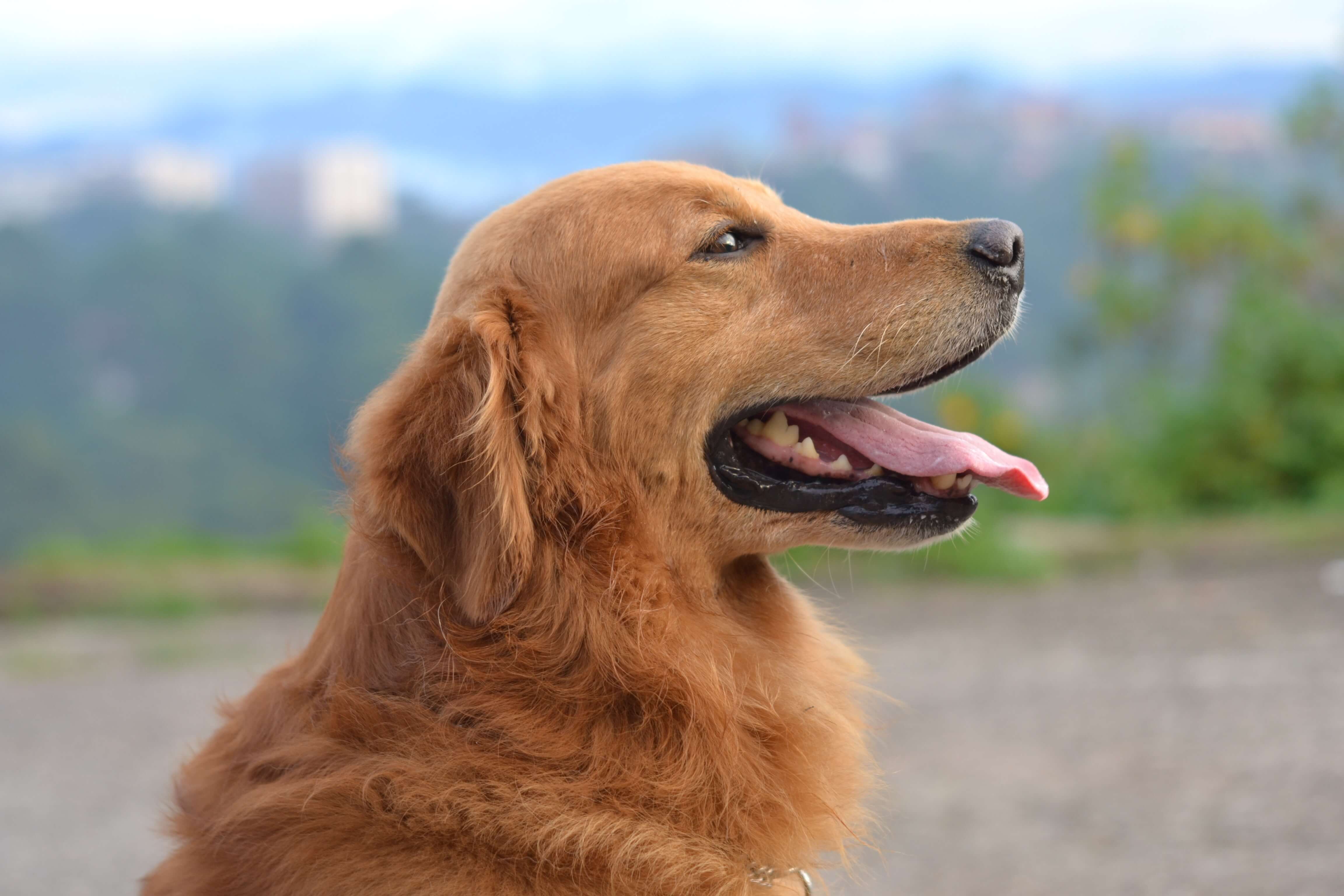
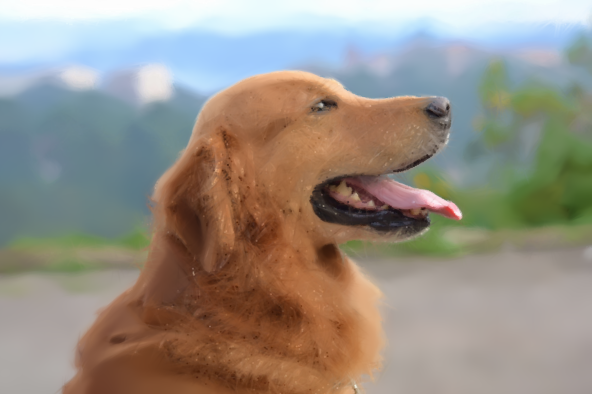
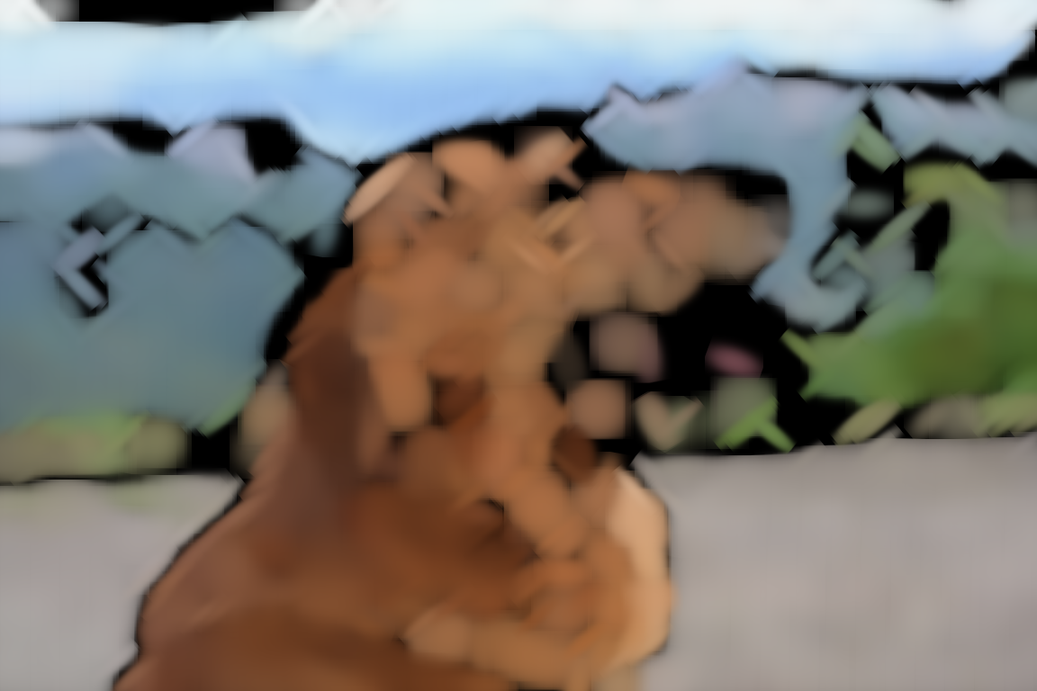
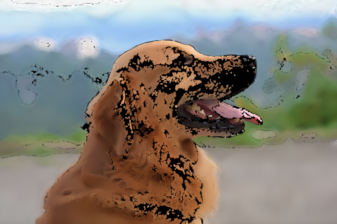
We test the feature extraction algorithm on the following image.

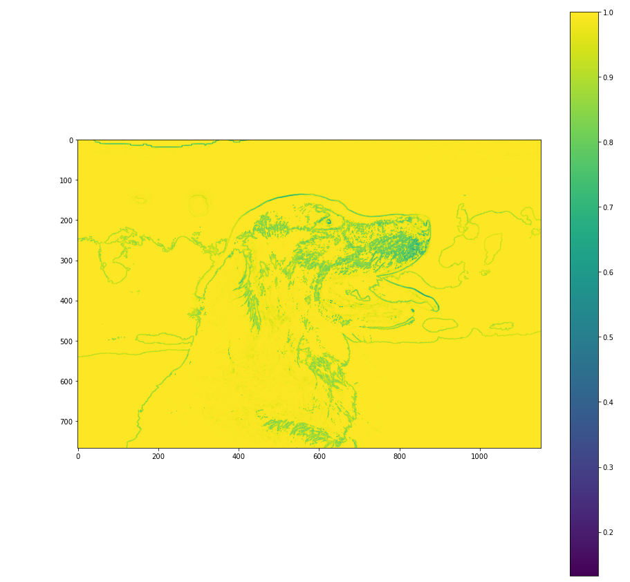
The maximum activation of all filters at each location in the image is shown below.

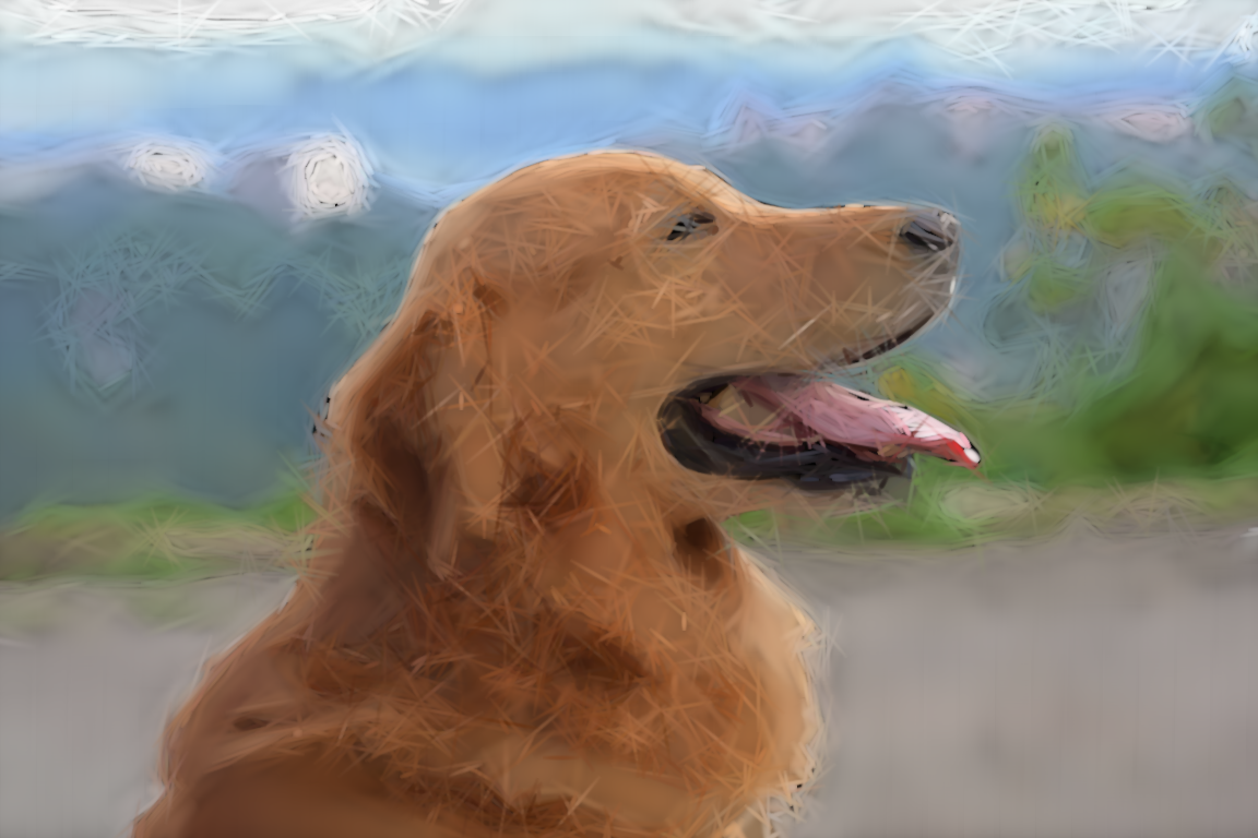
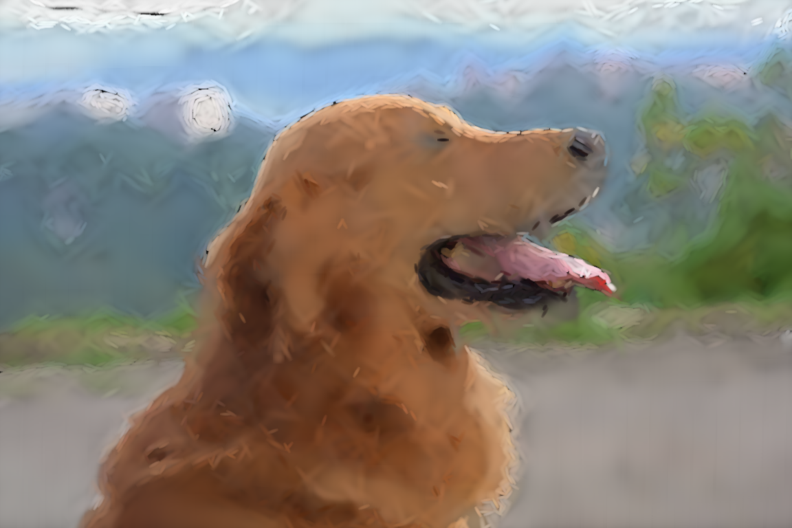
After we run convolution on the image we get a tensor where each value represents how well the filter activated at the current location. Once we extract features in the image, we can reconstruct the image by only selecting features with high activation scores, and redraw those features on a new blank image. We “compress” the representation by iteratively selecting the highest activated filters in locations that have not been colored already, in order to avoid recoloring the same regions with the same color. There are plenty of different ways to do this with many knobs to turn, and each method yields a slightly different image. For each method, if we draw N features extracted from an image with M pixels, then we loosely consider the compression rate to be M/N (waving our hands a bit — the real compression rate is a bit more complicated than that). The code for this project can be found on github. The images below show outputs of the algorithm using different methods for reconstructing the image, along with their compression rates.

Lastly, I would like to highlight the elegance of representing datapoints on a hypersphere. If we interpret the magnitude of a point as the certainty of the location of the point, and the direction as the features of the point, then taking the average point of a set of points is a simple and efficient way of summarizing the set of points - the average point describes roughly what direction the points are in, and by how much they converge. In other words, the average point of points in a hypersphere is a clean and compact way of capturing the mean and variance of the set of points.